pma - Performance Monitor Analyzer

What is pma, and what does it do?

The purpose of pma is to monitor, assess and (if necessary) identify corrective measures to address performance problems on Linux/UNIX systems. To do this, 3 utilities are required:

pmc - Performance Monitor Collector: a shell script that collects performance data (e.g., iostat, vmstat, and sar) into a (.pmc data) file. Download pmc from the pma github repository.
pma - Performance Monitor Analyzer: a C program that parses pmc's output performance data (.pmc) file(s) and produces output that can be graphed. Download pma from github.
xgraph - a graphing utility (the best one identified in antiquity) to display the output in a useful format. (Thanks to USC for hosting this link, but xgraph can be found in many places on the web.) Note: xgraph was not written by YOSJ staff.

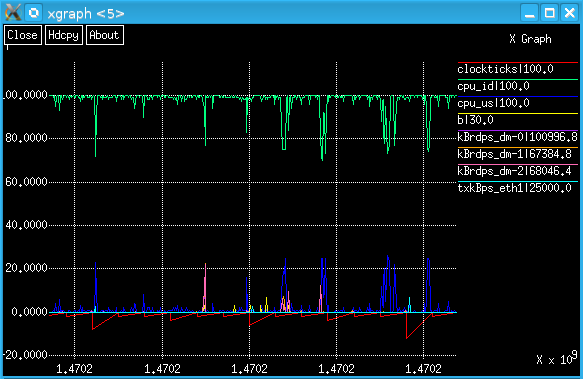
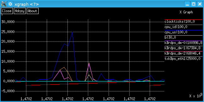
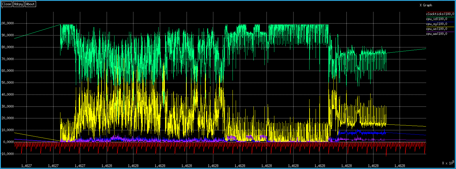
Sample Screen Shots of Data Collected by pmc, Processed by pma, and Graphed with xgraph

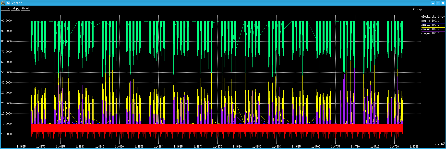
Above is a graph of the 4 CPU metrics: cpu_id, cpu_sy, cpu_us and cpu_wa, (and "clockticks") over a 16 week period of a lightly loaded Linux server. In this case, data has only been collected from 08:00 to 18:00 on weekdays.

However, graphing no more than a week's worth of data is recommended (due to limitations of xgraph).

Above is one week's data (Mon-Fri) from the same Linux server using the same CPU metrics as before (and "clockticks").

Above shows 2 CPU metrics and some others (and "clockticks") during the same week on the same Linux server.

Zoomed in on Wed.

10:00 to 12:00 Wed.

A 5 minute period of particular interest.

'clockticks'??? 1.4702???

If you've got this far, you're probably wondering:

What's the story with this odd 'clockticks' metric?, and
What are these preposterous numbers on the x (time) axis?

About xgraph

Sadly, xgraph cannot display formatted date/time values (e.g., "20231231 14:55:10"), but it can handle time in seconds "correctly" (i.e., linear, monotonically increasing). The problem, of course, is that there are a rather lot of seconds since "the Epoch". Adding a 'clockticks' pseudo-metric is the method developed to provide the time axis information in a readable format.

No graphing utility has yet been identified that can handle date/time axis elegantly and also performs as well as xgraph in all other important ways - e.g., xgraph's zooming capability.

General pma Information

Of course there are many products and applications to monitor Linux/UNIX performance, but... Perhaps you don't have one already. Maybe you have one, but it doesn't do what you need. Maybe you have one you like and use regularly, but you can't install the agent it requires (for whatever reason). Perchance you want to modify it - so it does exactly what you need! In such cases, pmc, pma and xgraph can be of use; all 3 can run as any user - no root access is required!

Theoretically, one could graph all the vmstat metrics, iostat metrics (per disk!) and (for Linux) sar -n DEV metrics (per interface!) - plus 'clockticks' (see below) - on the same graph. However, xgraph (when compiled on Linux) can't handle it, and - even if it could - the output would be unreadable with too many "curves". Therefore, it's better to graph no more than the number of lines one can see clearly.

Actually, pma can be used to analyze any data that's formatted in "pma format". (Which - by amazing happenstance - is precisely the format that pmc generates!) That is, it doesn't have to be *nix data, or even computer data - it can be any data whatsoever. (See the pollinators page below.)

'clockticks' Explained

The first thing to point out is that clockticks are configurable. The default configuration (level values) is shown below..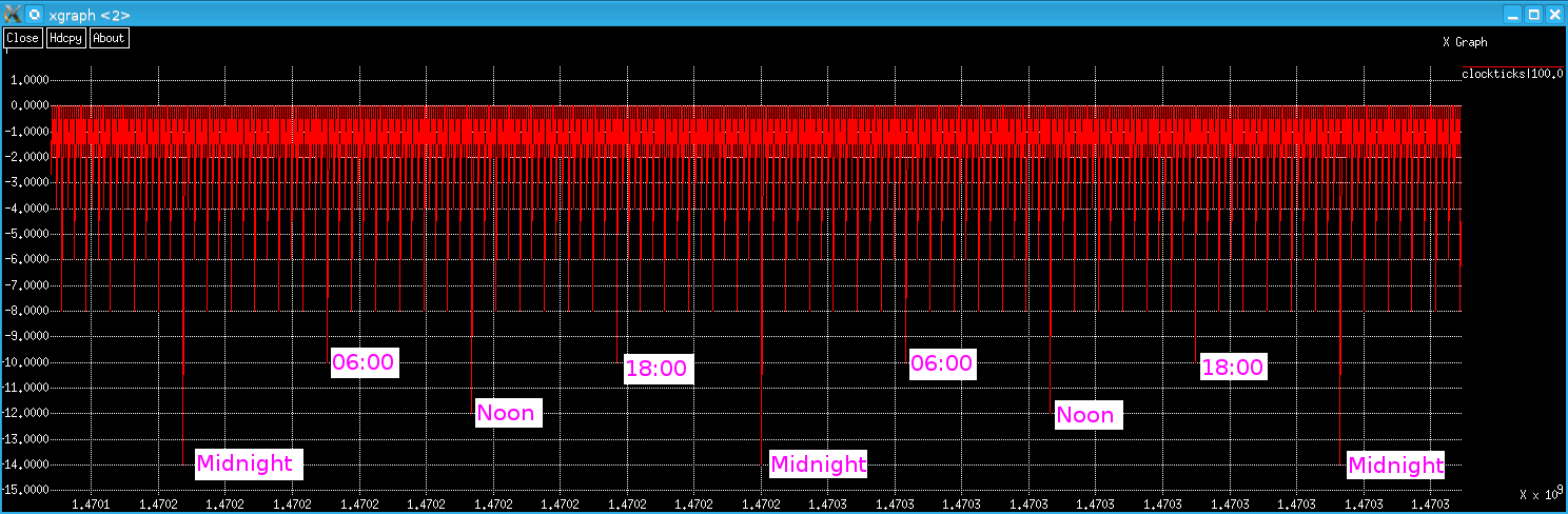

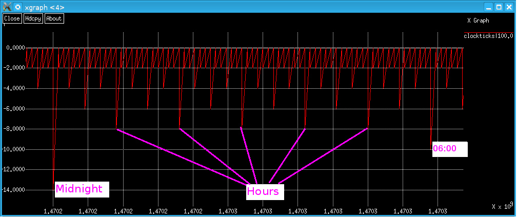
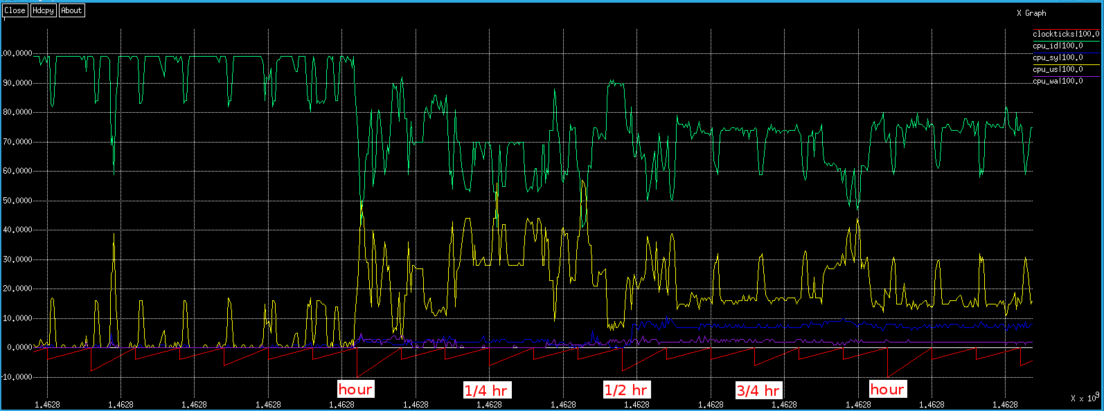
Above shows data collected over a period of about 3 days. Note the midnight 'clockticks' are the smallest values (-14).

Above shows about 14 hours of data (from 23:00 to 13:00 the next day).

Zooming in on 'clockticks' (above), note that the y values are: hours: -10, half hours: -8, quarter hours: -6, and every 5 minutes: -4. (Note: not default values.)

Here is some CPU data collected (and 'clockticks') during an interval lasting about 17 hours.

Clockticks intervals are configurable. In v0.0.1, there were 6 "levels". The screenshots above show clockticks using 5 levels: 24h, 1h, 30m, 15m and 5 min. As of v0.0.2, there are 8 levels, and the 7 default clockticks intervals are: 24h, 12h, 6h, 1h, 30m, 15, and 5m. But one can set the interval for any level to any value, as long as they are divisible by the higher levels.

Usage Notes

xgraph is a fantastic utility. One can zoom to an arbitrarily small scale. However, for this particular application, it would be better if the time axis could be displayed in a date_time format. (If anyone knows of a better alternative to xgraph, please let me know!)
You kind of have to know where you're looking (in the data). In practice, this is not difficult.
Excel was evaluated as a graphing tool - both in antiquity and recently. It simply cannot handle graphs with a lot of data. The same is true of LibreOffice Calc.
The above screen shots are real data from real systems.
By default, the pmc (Performance Monitor Collector) shell script produces output from vmstat and iostat using only the time and interval options. On Linux, pmc also runs sar -n DEV - also with only the time and interval value arguments. The output of these commands is transformed slightly into the format that pma requires. pmc could be modified, but if pma is to analyze the data, pmc must still produce output in the format pma requires ("pma format").
For Linux, the metrics that pmc produces are:
- vmstat: r b swpd free buff cache si so bi bo in cs us sy id wa st
- iostat (per device): tps kB_read/s kB_wrtn/s kB_read kB_wrtn
- sar -n DEV (per device): rxpck/s txpck/s rxkB/s txkB/s rxcmp/s txcmp/s rxmcst/s (Fedora 23 also has %ifutil)
See the Linux and/or UNIX man pages for the metric definitions (e.g., for vmstat, iostat, and sar).
pmc divides data into classes (e.g., VM, IO, and NET). Classes must have metrics. Some class' metrics also have devices. For example, VM metrics (such as 'free') do not have an associated device - so VM has been termed a 'vector class'. The IO class can (and generally does) have multiple devices (e.g., disks, logical volumes, optical drives, etc.). So, each metric has one or more associated devices. For example, tps for sda, sdb, dm-0, etc. Such classes are called 'array classes'. These have 'metric_device' values (one per device), as well as a metric value for all of the devices combined - e.g., tps, and tps_sda, tps_sdb.... (NET is also an array class.) To recap:
- Vector classes (VM for vmstat data) have metrics (e.g., free), but do not have (subordinate) metric_devices.
- Array classes (IO for iostat data and NET for sar -n DEV data) have metrics (e.g., tps), and they also have (subordinate) metric_devices - e.g., tps_sda, where tps is the metric and sda is the device.
pma requires that metric names be unique - even across classes. For example, pma does not allow an IO metric named 'sy' if there is also a VM metric named 'sy' (as is the case on AIX). For this reason (and for added clarity), naming the VM CPU metrics ('us', 'sy', 'id' and 'wa') as 'cpu_us', 'cpu_sy', 'cpu_id' and 'cpu_wa' is recommended.
Because pma adapts to the data, one can change the metric names (in pmc) nearly arbitrarily (see below for some restrictions). For example, "r b ... wa st" could be changed to "fred barney ... wilma betty" (though I don't advocate these particular choices, as they're patently silly!) - as long as there are the correct number of them (17, in this case).
pma can produce either or both of two types of output:
- "multiple files directory mode" ('-m multiple_files_directory_name'): The directory specified is created (if it doesn't exist) and one file for each metric(s) and/or metric_device(s) specified (in the config_file) is created and populated.
- "single output file mode" ('-s single_output_file_name'): The file specified is created (if it doesn't exist) and populated with the metric(s) and/or metric_device(s) specified (in the config_file) - separated by a separator character - e.g., a CSV file.
pma has several configuration parameters that allow (using both '-m' and '-s' output file formats) different types of output files to be generated - e.g., for a graphing tool other than xgraph - should a suitable one ever be identified.
When using "multiple file directory mode" ('-m') - where pma The slash ('/') character is a particularly bad choice for Linux/UNIX file names, so it's generally a good idea to replace all 'foo/s' (foos per second) with 'foops'. White-space (tab and space) in metric names (e.g., "part1 part2") is also not supported.
pma always calculates statistics for all metrics and metric_devices (maximum, average and count), whether they are output or not. This data is displayed with the '-d' (data) option.
pma displays parameter information with the '-p' option.
Determining which data - metric(s) and/or metric_device(s) - is output works as follows:
- pma initializes all metrics and device_metrics scale values to 0.
- Metric's and device_metric's scale values are optionally set in the configuration file.
- The configuration file is processed in (top to bottom) order.
- If the scale value of a metric that has subordinate device(s) - i.e., an array class metric - is set, all of that metric's subordinate metric_device(s) are also set to this value.
- These subordinate metric_device(s) may be individually set to different values - including 0, of course.
- Metrics that have a 0 scale value are not output.
Log files can get fairly large, so pmc allows optional start and stop hours. Entire days (e.g., "Sat" and/or "Sun") can also optionally be skipped.
The ancestors of pmc and pma (together with xgraph) have been extremely useful many times over the years.
Obviously, the OS utilities producing the raw data (e.g., vmstat, iostat and sar) must be installed on the system(s) being analyzed.
Analysis need not be performed on the system where the data is collected, of course. So, you could email someone the link to pmc and the command to invoke it, get them to email you back the output file(s), and then analyze the data on your system.
AFAIK, if you feed pma a valid (.pmc data) file as its input, it will run successfully and produce correct output.
pmc is a shell script, so it should on most (all?) *NIX platforms.
pma has been tested on SLES, OpenSUSE, Fedora, AIX and Cygwin.
If a better graphing utility becomes available, 'clockticks' could be jettisoned and the x (time) axis could be made to display meaningful values.
To get xgraph to compile, I renamed 'getline' to 'xgraph_getline' in dialog.c.
Depending on the platform, xgraph can core dump if its given too many "curves" to graph. It's hard to see what's happening with too many, so don't graph more than about 10 at a time.
Let me know if I have made any outrageously incorrect statements, and I'll correct them accordingly.

Using pmc, pma and xgraph to Display Performance Metrics

pmc (Performance Monitor Collector)

pmc is a simple shell script that runs native Linux/UNIX commands vmstat, iostat and sar and (with some simple text post-processing) logs this data to text (.pmc data) file(s).

The pmc Usage Message

$ pmc usage: pmc [OPTION ...] -o outputfilepattern [defaults:] WHERE: -o outfilepattern output log file pattern/name none (required!) OPTIONs are: -f first_hour first hour to collect data 0 -l last_hour last hour to collect data 23 -c count count parameter 12 -i interval interval parameter 10 -d disk/disk_list disk or 'disk1 ... diskN' to INclude none (all disks) -x day/day_list week day or 'day1 ... dayN' to EXclude none -V Do NOT collect vmstat output collect data -I Do NOT collect iostat output collect data -N Do NOT collect sar -n output collect data -v display the version of pmc -h display this usage message e.g.: pmc -o logfile pmc -f 9 -l 17 -o logfile pmc -f 9 -l 17 -d sda -d sdb -x Sat -x Sun -o logfile pmc -f 7 -l 19 -d 'dm-3 dm-6' -o logfile For a single date-stamped log file (no quotes): pmc [OPTION ...] -o $(hostname)_$(date +%Y%m%d.pmc) For a new date-stamped log file each day (single quotes): pmc [OPTION ...] -o '$(hostname)_$(date +%Y%m%d.pmc)'

pma (Performance Monitor Analyzer)

pma is a C program that transforms the (.pmc data) file(s) generated by pmc into a format that is suitable for performance analysis. In particular, it produces output that can be graphed with xgraph.

The pma Usage Message

How to use pmc, pma and xgraph

Start collecting data:

$ nohup pmc -o hostA.pmc &
Wait ... Once you have some data...
Run pma the first time to generate a configuration file "template". Note: pma's '-p' option displays the (active and default) parameter values, and the '-d' option displays the data summary values (maximum, average, and "count" - AKA number of data values):

$ pma -pd hostA.pmc > config_file W: no output file has been specified!
pma issues a suitable warning.

Below is a sample config_file. Note that all the lines are comments (they start with '#'):
# Parameter Active Value Default Value # ------------------------- ------------------------- ------------------------- # fullscale '100.0' # '100.0' # TZ '' # '' # metricdeviceseparator '_' # '_' # singlefiledateformat '%x %X' # '%x %X' # singlefiledelimiter ',' # ',' # multifiledateformat '%s' # '%s' # multifiledelimiter ' ' # ' ' # multifileheaderformat '"%s|%.1f"' # '"%s|%.1f"' # clockticksfilename 'clockticks' # 'clockticks' # clockticks_level_0 '86400' # '86400' # clockticks_level_1 '43200' # '43200' # clockticks_level_2 '21600' # '21600' # clockticks_level_3 '3600' # '3600' # clockticks_level_4 '1800' # '1800' # clockticks_level_5 '900' # '900' # clockticks_level_6 '300' # '300' # clockticks_level_7 '0' # '0' ### Summary Data ################### Max ################# Avg ######### Num # r 13.0 # 1.1 3817 # b 3.0 # 0.0 3817 # swpd 36692.0 # 36690.8 3817 # free 636456.0 # 540151.0 3817 # buff 737148.0 # 728858.4 3817 # cache 8757440.0 # 8718379.5 3817 # si 0.0 # 0.0 3817 # so 0.0 # 0.0 3817 # bi 23185.0 # 103.9 3817 # bo 19393.0 # 178.5 3817 # in 3128.0 # 1977.1 3817 # cs 15840.0 # 4883.2 3817 # cpu_us 94.0 # 21.9 3817 # cpu_sy 17.0 # 2.7 3817 # cpu_id 96.0 # 74.5 3817 # cpu_wa 44.0 # 0.8 3817 # st 0.0 # 0.0 3817 # tps 4426.6 # 2.3 95425 ## tps_sda 275.3 ## 17.3 3817 ## tps_sdb 702.6 ## 4.9 3817 ## tps_dm-0 41.8 ## 5.9 3817 ## tps_dm-1 0.0 ## 0.0 3817 ## tps_dm-2 0.0 ## 0.0 3817 ## tps_dm-3 0.3 ## 0.0 3817 ## tps_dm-4 36.0 ## 0.1 3817 ## tps_dm-5 157.6 ## 4.9 3817 ## tps_dm-6 112.4 ## 3.2 3817 ## tps_dm-7 155.5 ## 2.4 3817 ## tps_dm-8 82.1 ## 2.5 3817 ## tps_dm-9 4426.6 ## 5.8 3817 ## tps_dm-10 184.7 ## 2.4 3817 ## tps_dm-11 122.6 ## 1.1 3817 ## tps_dm-12 702.3 ## 1.4 3817 ## tps_dm-13 160.6 ## 1.3 3817 ## tps_dm-14 0.0 ## 0.0 3817 ## tps_dm-15 0.0 ## 0.0 3817 ## tps_dm-16 35.3 ## 1.5 3817 ## tps_dm-17 244.4 ## 2.4 3817 ## tps_dm-18 0.0 ## 0.0 3817 ## tps_dm-19 7.6 ## 0.0 3817 ## tps_dm-20 2.2 ## 0.0 3817 ## tps_dm-21 0.0 ## 0.0 3817 ## tps_sr0 0.0 ## 0.0 3817 # kBrdps 45899.4 # 16.6 95425 ## kBrdps_sda 35811.7 ## 147.8 3817 ## kBrdps_sdb 25320.0 ## 60.1 3817 ## kBrdps_dm-0 148.8 ## 0.1 3817 ## kBrdps_dm-1 0.0 ## 0.0 3817 ## kBrdps_dm-2 0.0 ## 0.0 3817 ## kBrdps_dm-3 0.8 ## 0.0 3817 ## kBrdps_dm-4 259.2 ## 0.1 3817 ## kBrdps_dm-5 35723.0 ## 88.3 3817 ## kBrdps_dm-6 35077.3 ## 21.2 3817 ## kBrdps_dm-7 0.7 ## 0.0 3817 ## kBrdps_dm-8 0.7 ## 0.0 3817 ## kBrdps_dm-9 0.8 ## 0.0 3817 ## kBrdps_dm-10 45899.4 ## 48.4 3817 ## kBrdps_dm-11 2481.6 ## 12.7 3817 ## kBrdps_dm-12 11236.8 ## 16.1 3817 ## kBrdps_dm-13 25220.8 ## 19.2 3817 ## kBrdps_dm-14 0.0 ## 0.0 3817 ## kBrdps_dm-15 0.0 ## 0.0 3817 ## kBrdps_dm-16 0.0 ## 0.0 3817 ## kBrdps_dm-17 1897.6 ## 1.5 3817 ## kBrdps_dm-18 0.0 ## 0.0 3817 ## kBrdps_dm-19 568.8 ## 0.2 3817 ## kBrdps_dm-20 0.0 ## 0.0 3817 ## kBrdps_dm-21 0.0 ## 0.0 3817 ## kBrdps_sr0 0.0 ## 0.0 3817 # kBwtps 35410.5 # 28.6 95425 ## kBwtps_sda 14041.0 ## 222.4 3817 ## kBwtps_sdb 35377.7 ## 134.5 3817 ## kBwtps_dm-0 334.4 ## 47.3 3817 ## kBwtps_dm-1 0.0 ## 0.0 3817 ## kBwtps_dm-2 0.0 ## 0.0 3817 ## kBwtps_dm-3 2.4 ## 0.0 3817 ## kBwtps_dm-4 62.4 ## 0.8 3817 ## kBwtps_dm-5 6956.4 ## 38.4 3817 ## kBwtps_dm-6 2624.3 ## 39.3 3817 ## kBwtps_dm-7 6930.0 ## 24.0 3817 ## kBwtps_dm-8 2598.7 ## 24.9 3817 ## kBwtps_dm-9 35410.5 ## 46.1 3817 ## kBwtps_dm-10 6009.6 ## 59.1 3817 ## kBwtps_dm-11 804.0 ## 12.8 3817 ## kBwtps_dm-12 1175.2 ## 15.0 3817 ## kBwtps_dm-13 1008.0 ## 17.8 3817 ## kBwtps_dm-14 0.0 ## 0.0 3817 ## kBwtps_dm-15 0.0 ## 0.0 3817 ## kBwtps_dm-16 282.4 ## 11.8 3817 ## kBwtps_dm-17 1955.2 ## 19.1 3817 ## kBwtps_dm-18 0.0 ## 0.0 3817 ## kBwtps_dm-19 13.6 ## 0.0 3817 ## kBwtps_dm-20 17.6 ## 0.4 3817 ## kBwtps_dm-21 0.0 ## 0.0 3817 ## kBwtps_sr0 0.0 ## 0.0 3817 # kBrd 458994.0 # 166.3 95425 ## kBrd_sda 358117.0 ## 1477.7 3817 ## kBrd_sdb 253200.0 ## 601.5 3817 ## kBrd_dm-0 1488.0 ## 0.8 3817 ## kBrd_dm-1 0.0 ## 0.0 3817 ## kBrd_dm-2 0.0 ## 0.0 3817 ## kBrd_dm-3 8.0 ## 0.0 3817 ## kBrd_dm-4 2592.0 ## 1.3 3817 ## kBrd_dm-5 357230.0 ## 882.6 3817 ## kBrd_dm-6 350773.0 ## 212.0 3817 ## kBrd_dm-7 7.0 ## 0.0 3817 ## kBrd_dm-8 7.0 ## 0.0 3817 ## kBrd_dm-9 8.0 ## 0.0 3817 ## kBrd_dm-10 458994.0 ## 484.4 3817 ## kBrd_dm-11 24816.0 ## 127.3 3817 ## kBrd_dm-12 112368.0 ## 161.5 3817 ## kBrd_dm-13 252208.0 ## 192.5 3817 ## kBrd_dm-14 0.0 ## 0.0 3817 ## kBrd_dm-15 0.0 ## 0.0 3817 ## kBrd_dm-16 0.0 ## 0.0 3817 ## kBrd_dm-17 18976.0 ## 14.6 3817 ## kBrd_dm-18 0.0 ## 0.0 3817 ## kBrd_dm-19 5688.0 ## 1.8 3817 ## kBrd_dm-20 0.0 ## 0.0 3817 ## kBrd_dm-21 0.0 ## 0.0 3817 ## kBrd_sr0 0.0 ## 0.0 3817 # kBwt 354105.0 # 285.6 95425 ## kBwt_sda 140410.0 ## 2224.4 3817 ## kBwt_sdb 353777.0 ## 1345.2 3817 ## kBwt_dm-0 3344.0 ## 472.9 3817 ## kBwt_dm-1 0.0 ## 0.0 3817 ## kBwt_dm-2 0.0 ## 0.0 3817 ## kBwt_dm-3 24.0 ## 0.0 3817 ## kBwt_dm-4 624.0 ## 8.0 3817 ## kBwt_dm-5 69564.0 ## 384.1 3817 ## kBwt_dm-6 26243.0 ## 393.4 3817 ## kBwt_dm-7 69300.0 ## 239.9 3817 ## kBwt_dm-8 25987.0 ## 249.4 3817 ## kBwt_dm-9 354105.0 ## 461.4 3817 ## kBwt_dm-10 60096.0 ## 591.2 3817 ## kBwt_dm-11 8040.0 ## 128.0 3817 ## kBwt_dm-12 11752.0 ## 150.5 3817 ## kBwt_dm-13 10080.0 ## 177.9 3817 ## kBwt_dm-14 0.0 ## 0.0 3817 ## kBwt_dm-15 0.0 ## 0.0 3817 ## kBwt_dm-16 2824.0 ## 117.9 3817 ## kBwt_dm-17 19552.0 ## 191.1 3817 ## kBwt_dm-18 0.0 ## 0.0 3817 ## kBwt_dm-19 136.0 ## 0.1 3817 ## kBwt_dm-20 176.0 ## 3.9 3817 ## kBwt_dm-21 0.0 ## 0.0 3817 ## kBwt_sr0 0.0 ## 0.0 3817 # rxpkps 11566.9 # 93.5 8328 ## rxpkps_lo 11566.9 ## 179.6 4164 ## rxpkps_eth0 88.6 ## 7.3 4164 # txpkps 11566.9 # 92.3 8328 ## txpkps_lo 11566.9 ## 179.6 4164 ## txpkps_eth0 91.4 ## 5.0 4164 # rxkBps 3965.8 # 45.6 8328 ## rxkBps_lo 3965.8 ## 89.3 4164 ## rxkBps_eth0 69.5 ## 1.9 4164 # txkBps 3965.8 # 45.2 8328 ## txkBps_lo 3965.8 ## 89.3 4164 ## txkBps_eth0 36.8 ## 1.1 4164 # rxcmps 0.0 # 0.0 8328 ## rxcmps_lo 0.0 ## 0.0 4164 ## rxcmps_eth0 0.0 ## 0.0 4164 # txcmps 0.0 # 0.0 8328 ## txcmps_lo 0.0 ## 0.0 4164 ## txcmps_eth0 0.0 ## 0.0 4164 # rxmctps 0.0 # 0.0 8328 ## rxmctps_lo 0.0 ## 0.0 4164 ## rxmctps_eth0 0.0 ## 0.0 4164
Edit the config_file. The aim of the game here is to scale the metrics so they can all be displayed on the same graph. Sometimes, r and b will be less than 5, but memory parameters will be in the millions. The idea is scale all the metrics by setting scale values (for each) that would be 100 on the graph if you had a data point of that value. Recommendation: round up each metric's scale value to a number that's easy to divide in your head. (Note: the maximum scale value need not be 100. One can set a different value using the fullscale parameter, but the default of 100 is easy to divide.)
- Here is a sample config_file:
  
  # Parameter Active Value Default Value # ------------------------- ------------------------- ------------------------- # fullscale '100.0' # '100.0' # TZ '' # '' # metricdeviceseparator '_' # '_' # singlefiledateformat '%x %X' # '%x %X' # singlefiledelimiter ',' # ',' # multifiledateformat '%s' # '%s' # multifiledelimiter ' ' # ' ' # multifileheaderformat '"%s|%.1f"' # '"%s|%.1f"' # clockticksfilename 'clockticks' # 'clockticks' # clockticks_level_0 '86400' # '86400' # clockticks_level_1 '43200' # '43200' # clockticks_level_2 '21600' # '21600' # clockticks_level_3 '3600' # '3600' # clockticks_level_4 '1800' # '1800' # clockticks_level_5 '900' # '900' # clockticks_level_6 '300' # '300' # clockticks_level_7 '0' # '0' ### Summary Data ################### Max ################# Avg ######### Num r 20.0 # 1.1 3817 b 20.0 # 0.0 3817 # swpd 36692.0 # 36690.8 3817 # free 636456.0 # 540151.0 3817 # buff 737148.0 # 728858.4 3817 # cache 8757440.0 # 8718379.5 3817 # si 0.0 # 0.0 3817 # so 0.0 # 0.0 3817 # bi 23185.0 # 103.9 3817 # bo 19393.0 # 178.5 3817 # in 3128.0 # 1977.1 3817 # cs 15840.0 # 4883.2 3817 cpu_us 100.0 # 21.9 3817 cpu_sy 100.0 # 2.7 3817 cpu_id 100.0 # 74.5 3817 cpu_wa 100.0 # 0.8 3817 # st 0.0 # 0.0 3817 tps 5000.0 # 2.3 95425 ## tps_sda 275.3 ## 17.3 3817 ## tps_sdb 702.6 ## 4.9 3817 ## tps_dm-0 41.8 ## 5.9 3817 ## tps_dm-1 0.0 ## 0.0 3817 ## tps_dm-2 0.0 ## 0.0 3817 ## tps_dm-3 0.3 ## 0.0 3817 ## tps_dm-4 36.0 ## 0.1 3817 ## tps_dm-5 157.6 ## 4.9 3817 ## tps_dm-6 112.4 ## 3.2 3817 ## tps_dm-7 155.5 ## 2.4 3817 ## tps_dm-8 82.1 ## 2.5 3817 ## tps_dm-9 4426.6 ## 5.8 3817 ## tps_dm-10 184.7 ## 2.4 3817 ## tps_dm-11 122.6 ## 1.1 3817 ## tps_dm-12 702.3 ## 1.4 3817 ## tps_dm-13 160.6 ## 1.3 3817 ## tps_dm-14 0.0 ## 0.0 3817 ## tps_dm-15 0.0 ## 0.0 3817 ## tps_dm-16 35.3 ## 1.5 3817 ## tps_dm-17 244.4 ## 2.4 3817 ## tps_dm-18 0.0 ## 0.0 3817 ## tps_dm-19 7.6 ## 0.0 3817 ## tps_dm-20 2.2 ## 0.0 3817 ## tps_dm-21 0.0 ## 0.0 3817 ## tps_sr0 0.0 ## 0.0 3817 kBrdps 50000.0 # 16.6 95425 ## kBrdps_sda 35811.7 ## 147.8 3817 ## kBrdps_sdb 25320.0 ## 60.1 3817 ## kBrdps_dm-0 148.8 ## 0.1 3817 ## kBrdps_dm-1 0.0 ## 0.0 3817 ## kBrdps_dm-2 0.0 ## 0.0 3817 ## kBrdps_dm-3 0.8 ## 0.0 3817 ## kBrdps_dm-4 259.2 ## 0.1 3817 ## kBrdps_dm-5 35723.0 ## 88.3 3817 ## kBrdps_dm-6 35077.3 ## 21.2 3817 ## kBrdps_dm-7 0.7 ## 0.0 3817 ## kBrdps_dm-8 0.7 ## 0.0 3817 ## kBrdps_dm-9 0.8 ## 0.0 3817 ## kBrdps_dm-10 45899.4 ## 48.4 3817 ## kBrdps_dm-11 2481.6 ## 12.7 3817 ## kBrdps_dm-12 11236.8 ## 16.1 3817 ## kBrdps_dm-13 25220.8 ## 19.2 3817 ## kBrdps_dm-14 0.0 ## 0.0 3817 ## kBrdps_dm-15 0.0 ## 0.0 3817 ## kBrdps_dm-16 0.0 ## 0.0 3817 ## kBrdps_dm-17 1897.6 ## 1.5 3817 ## kBrdps_dm-18 0.0 ## 0.0 3817 ## kBrdps_dm-19 568.8 ## 0.2 3817 ## kBrdps_dm-20 0.0 ## 0.0 3817 ## kBrdps_dm-21 0.0 ## 0.0 3817 ## kBrdps_sr0 0.0 ## 0.0 3817 kBwtps 50000.0 # 28.6 95425 ## kBwtps_sda 14041.0 ## 222.4 3817 ## kBwtps_sdb 35377.7 ## 134.5 3817 ## kBwtps_dm-0 334.4 ## 47.3 3817 ## kBwtps_dm-1 0.0 ## 0.0 3817 ## kBwtps_dm-2 0.0 ## 0.0 3817 ## kBwtps_dm-3 2.4 ## 0.0 3817 ## kBwtps_dm-4 62.4 ## 0.8 3817 ## kBwtps_dm-5 6956.4 ## 38.4 3817 ## kBwtps_dm-6 2624.3 ## 39.3 3817 ## kBwtps_dm-7 6930.0 ## 24.0 3817 ## kBwtps_dm-8 2598.7 ## 24.9 3817 ## kBwtps_dm-9 35410.5 ## 46.1 3817 ## kBwtps_dm-10 6009.6 ## 59.1 3817 ## kBwtps_dm-11 804.0 ## 12.8 3817 ## kBwtps_dm-12 1175.2 ## 15.0 3817 ## kBwtps_dm-13 1008.0 ## 17.8 3817 ## kBwtps_dm-14 0.0 ## 0.0 3817 ## kBwtps_dm-15 0.0 ## 0.0 3817 ## kBwtps_dm-16 282.4 ## 11.8 3817 ## kBwtps_dm-17 1955.2 ## 19.1 3817 ## kBwtps_dm-18 0.0 ## 0.0 3817 ## kBwtps_dm-19 13.6 ## 0.0 3817 ## kBwtps_dm-20 17.6 ## 0.4 3817 ## kBwtps_dm-21 0.0 ## 0.0 3817 ## kBwtps_sr0 0.0 ## 0.0 3817 kBrd 500000.0 # 166.3 95425 ## kBrd_sda 358117.0 ## 1477.7 3817 ## kBrd_sdb 253200.0 ## 601.5 3817 ## kBrd_dm-0 1488.0 ## 0.8 3817 ## kBrd_dm-1 0.0 ## 0.0 3817 ## kBrd_dm-2 0.0 ## 0.0 3817 ## kBrd_dm-3 8.0 ## 0.0 3817 ## kBrd_dm-4 2592.0 ## 1.3 3817 ## kBrd_dm-5 357230.0 ## 882.6 3817 ## kBrd_dm-6 350773.0 ## 212.0 3817 ## kBrd_dm-7 7.0 ## 0.0 3817 ## kBrd_dm-8 7.0 ## 0.0 3817 ## kBrd_dm-9 8.0 ## 0.0 3817 ## kBrd_dm-10 458994.0 ## 484.4 3817 ## kBrd_dm-11 24816.0 ## 127.3 3817 ## kBrd_dm-12 112368.0 ## 161.5 3817 ## kBrd_dm-13 252208.0 ## 192.5 3817 ## kBrd_dm-14 0.0 ## 0.0 3817 ## kBrd_dm-15 0.0 ## 0.0 3817 ## kBrd_dm-16 0.0 ## 0.0 3817 ## kBrd_dm-17 18976.0 ## 14.6 3817 ## kBrd_dm-18 0.0 ## 0.0 3817 ## kBrd_dm-19 5688.0 ## 1.8 3817 ## kBrd_dm-20 0.0 ## 0.0 3817 ## kBrd_dm-21 0.0 ## 0.0 3817 ## kBrd_sr0 0.0 ## 0.0 3817 kBwt 500000.0 # 285.6 95425 ## kBwt_sda 140410.0 ## 2224.4 3817 ## kBwt_sdb 353777.0 ## 1345.2 3817 ## kBwt_dm-0 3344.0 ## 472.9 3817 ## kBwt_dm-1 0.0 ## 0.0 3817 ## kBwt_dm-2 0.0 ## 0.0 3817 ## kBwt_dm-3 24.0 ## 0.0 3817 ## kBwt_dm-4 624.0 ## 8.0 3817 ## kBwt_dm-5 69564.0 ## 384.1 3817 ## kBwt_dm-6 26243.0 ## 393.4 3817 ## kBwt_dm-7 69300.0 ## 239.9 3817 ## kBwt_dm-8 25987.0 ## 249.4 3817 ## kBwt_dm-9 354105.0 ## 461.4 3817 ## kBwt_dm-10 60096.0 ## 591.2 3817 ## kBwt_dm-11 8040.0 ## 128.0 3817 ## kBwt_dm-12 11752.0 ## 150.5 3817 ## kBwt_dm-13 10080.0 ## 177.9 3817 ## kBwt_dm-14 0.0 ## 0.0 3817 ## kBwt_dm-15 0.0 ## 0.0 3817 ## kBwt_dm-16 2824.0 ## 117.9 3817 ## kBwt_dm-17 19552.0 ## 191.1 3817 ## kBwt_dm-18 0.0 ## 0.0 3817 ## kBwt_dm-19 136.0 ## 0.1 3817 ## kBwt_dm-20 176.0 ## 3.9 3817 ## kBwt_dm-21 0.0 ## 0.0 3817 ## kBwt_sr0 0.0 ## 0.0 3817 # rxpkps 11566.9 # 93.5 8328 ## rxpkps_lo 11566.9 ## 179.6 4164 ## rxpkps_eth0 88.6 ## 7.3 4164 # txpkps 11566.9 # 92.3 8328 ## txpkps_lo 11566.9 ## 179.6 4164 ## txpkps_eth0 91.4 ## 5.0 4164 rxkBps 4000.0 # 45.6 8328 ## rxkBps_lo 3965.8 ## 89.3 4164 ## rxkBps_eth0 69.5 ## 1.9 4164 txkBps 4000.0 # 45.2 8328 ## txkBps_lo 3965.8 ## 89.3 4164 ## txkBps_eth0 36.8 ## 1.1 4164 # rxcmps 0.0 # 0.0 8328 ## rxcmps_lo 0.0 ## 0.0 4164 ## rxcmps_eth0 0.0 ## 0.0 4164 # txcmps 0.0 # 0.0 8328 ## txcmps_lo 0.0 ## 0.0 4164 ## txcmps_eth0 0.0 ## 0.0 4164 # rxmctps 0.0 # 0.0 8328 ## rxmctps_lo 0.0 ## 0.0 4164 ## rxmctps_eth0 0.0 ## 0.0 4164
- Uncomment all lines you might want to graph - remove the '#' character(s) at the start of these lines.
- Because they are percentage values, change all of the cpu_?? values you want to graph to 100.0.
- For each metric and/or metric_device that you might want to graph, use the maximum value that pma calculated on previous run(s) as the basis for the relevant scale value. I.e., round it up to something you can easily divide by fullscale (default is 100) in your head. In the above example, related parameters r and b have maximum values of 13 and 3, so a maximum scale of 20 would be a good choice for these parameters. If you might want to graph some/all of the tps_device metrics (with a maximum value for all of 4426.6), a sensible scale value would be 5000.
Run pma with your shiny new configuration file:

$ pma -c config_file -m Graph_Files hostA.pmc
Graph your files (CPU metrics, in this example):

$ xgraph -bg black -fg white Graph_Files/clockticks Graph_Files/cpu*
Note: 'clockticks' is the only time reference, so you should always graph that!
It should be possible (even if the xgraph output was unusably complicated) to graph all the metrics (and metric_device) curves on the same graph - like this:

$ xgraph -bg black -fg white Graph_Files/*
Unfortunately, xgraph dies if one attempts to graph too many metrics. The precise details are unknown. Graphing a relatively small number of "curves" works reliably (on the platforms tested so far).
Analyze your data to understand the problem(s) and design an action plan.
Apply your change(s).
Repeat until success is achieved.

More Examples

Use the standard input ('-') as the input:

$ pma -c config_file -m Graph_Files - < hostA.pmc
or
$ cat hostA.pmc | pma -c config_file -m Graph_Files -
Verbose mode warns of what always occurs if the first input file is stdin ('-'):

$ pma -vc config_file -m Graph_Files - < hostA.pmc i: First data set skipped when using - (stdin) as the FIRST input file
Note: This skipping is generally not a problem since there will be thousands of data sets.
Specify more than one input file:

$ pma -c config_file -m Graph_Files hostA_1.pmc hostA_2.pmc hostA_3.pmc
or

$ cat hostA_[123].pmc | pma -c config_file -m Graph_Files -
First files, then standard input (can't be more than one '-', and it must be last, for obvious reasons!):

$ pma -c config_file -m Graph_Files hostA_1.pmc hostA_2.pmc - < hostA_3.pmc
Send single file output to the screen - useful for testing:

$ pma -c config_file -s /dev/tty tiny_test_file.pmc

A Non-Linux/UNIX Example

The pollinators page demonstrates that pma really does adapt to the data, and that it can handle input files that are utterly unrelated to Linux/UNIX performance - as long as the data is in "pma format", of course..

The History of pma

pma is a complete rewrite (from scratch) of linuxperf - a program that has been used for many years to analyze the performance of Linux/UNIX systems.

With the older versions (like linuxperf), there was a dedicated version for each OS (e.g., Solaris, HP-UX, AIX). pma is different - it adapts to the data collected, so it can handle all of these OSs (though pmc would have to be trivially extended). In fact, it can handle a wide variety of data - as long as it conforms to pma's requirements. (See pollinators.)

For the pathologically over-curious, see the linuxperf page for details. But use pma, not linuxperf!