pma is the replacement for linuxperf!
Please do NOT use linuxperf!!!
In fact, I have taken down the linuxperf source code. But... for historical reference...Keen observers will note the strong external similarity with pma. There are a few subtle differences in how they work, but the big difference is that linuxperf is a one-trick pony - it only processes Linux output (as did its siblings, aixperf, solarisperf, etc.). In theory, pma can be used to graph lots of different types of data. See the pma page for details.
linuxperf
What is linuxperf, and what does it do?
The purpose of linuxperf is to monitor, assess and (if necessary) identify corrective measures to address performance problems on Linux systems. To do this, 3 utilities are required:- linuxperfmon - a trivial shell script that collects iostat and vmstat data into a log file.
- linuxperf - a C program that parses these log file(s) and produces output that can be graphed.
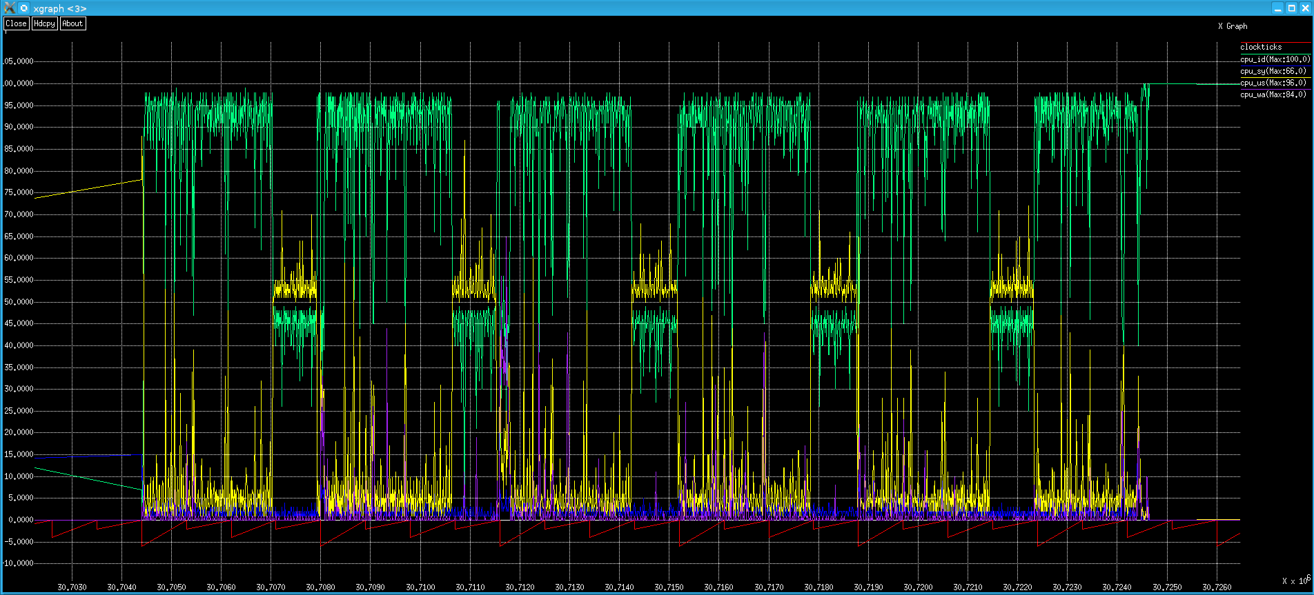
- xgraph - a graphing utility (the best one identified in antiquity) to display the output in a useful format. (Thanks to USC for hosting this link, but xgraph can be found in many places on the web.) Note: xgraph was not written by YOSJ Staff.
If you've got this far, you're probably wondering:
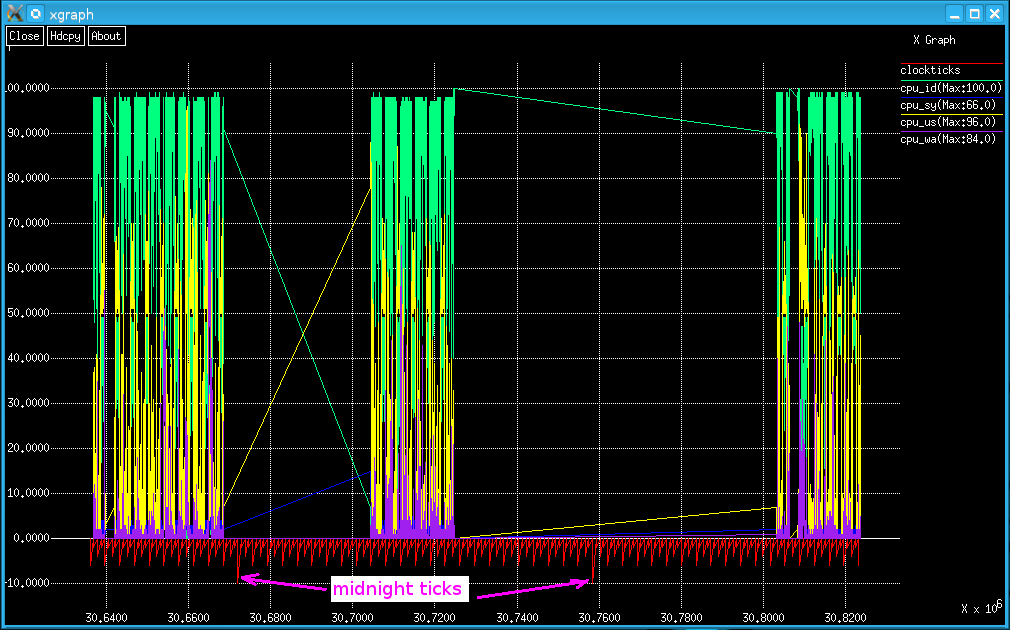
- What's the story with this odd "clockticks metric"?, and
- What are these preposterous numbers on the x (time) axis?
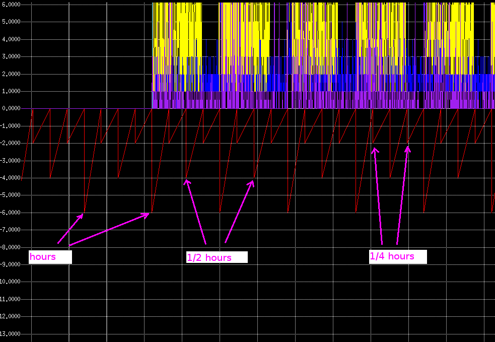
Notes:
- You kind of have to know where you're looking (in the data). In practice, this is very easy to do.
- xgraph is a fantastic utility. One can zoom to an arbitrarily small scale. However, for this particular application, it would be better if the time axis could be displayed in a date_time format.
- Though the attempt was several years ago, Excel was evaluated as a graphic tool. It was a dismal failure.
- It would be trivial to modify linuxperf to produce output for other graphing tool(s) - should a suitable one ever be identified.
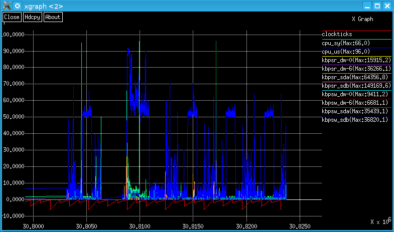
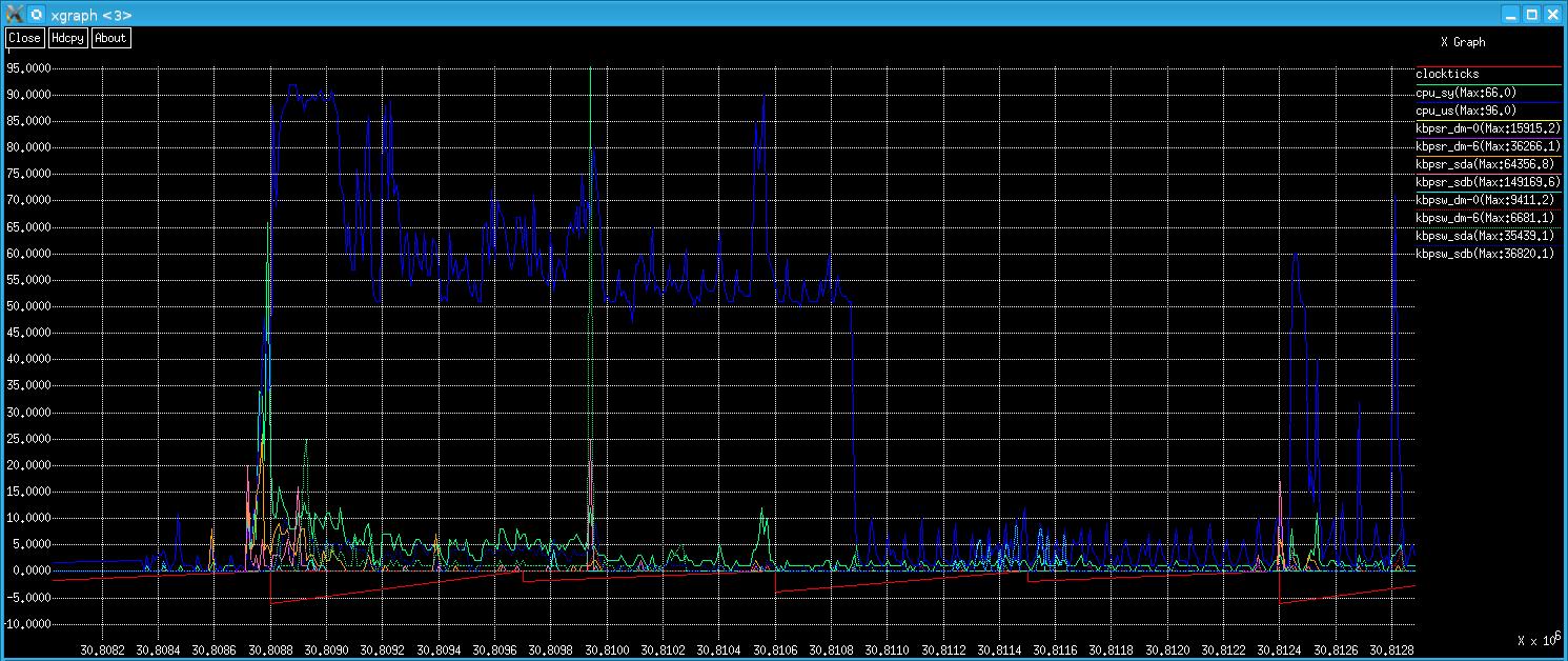
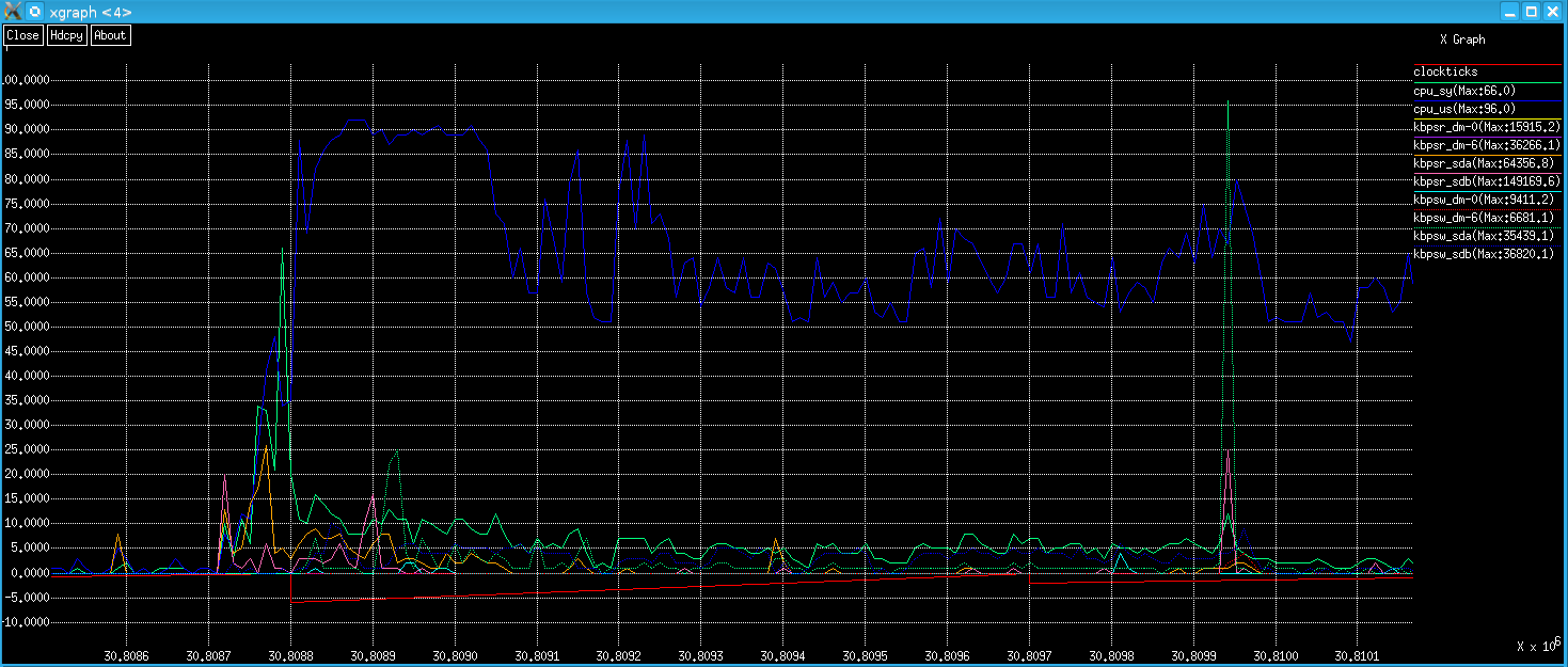
- The above screen shots are real data from a real system - albeit a lightly loaded one.
- Currently, linuxperfmon produces output from iostat and vmstat using only the time and iterations options.
This is also what linuxperf requires. If you change one, you'll have to change the other. These metrics are
as follows:
- vmstat: r b swpd free buff cache si so bi bo in cs us sy id wa st
- iostat (per device): tps kB_read/s kB_wrtn/s kB_read kB_wrtn
- Log files can get fairly large, so linuxperfmon currently allows start and stop hours. It also skips days "Sat" and "Sun". (Output is assumed to be in English.) It's left as a trivial exercise to be able to collect data on weekends and/or 24x7.
- These 3 tools have been extremely useful many times over the years. Every time a new performance bottleneck is encountered, a search ensued for something more useful. So far, these utilities have always proved to be the most effective analysis method identified.
- The fact that vmstat and iostat are often installed on Linux systems is also useful.
- Analysis need not be performed on the system where the data is collected, of course.
- linuxperf is a port from the AIX version, which came from the Tru64 version, which... (see history). If anybody is really keen to use linuxperf, it will need serious cleaning up. (This is about as far from my best code as one can get!)
- AFAIK, if you feed linuxperf a valid (input) log file, it will run successfully and produce correct output. If you feed linuxperf a corrupt (input) log file, it will die. This code definitely needs extra seat belts and airbags! You have been warned.
- It's only been tested on SLES, OpenSUSE and Fedora.
- If a better graphing utility becomes available, clockticks could be jettisoned and the x (time) axis could be made to display meaningful values.
- Currently, no network data is collected. If a suitable command is available that produces consistent output (including across various Linux versions), then it should be easy to add this functionality.
- To get xgraph to compile, I renamed 'getline' to 'xgraph_getline' in dialog.c.
- linuxperf also displays "text graphs". They're an anachronistic feature; if nothing else, they're good for a giggle.
How to use linuxperfmon, linuxperf and xgraph
- Start collecting data: nohup linuxperfmon log_file 7 22 [ disk ... ] &
- Wait ... Once you have some data...
- Run linuxperf the first time to create a config_file "template": linuxperf log_file > config_file
- Edit the config_file. The aim of the game here is to scale the metrics so they can all be displayed on the
same graph. Sometimes, r and b will be less than 5, but memory parameters will be in the millions. The idea is
scale all the metrics by setting maximum values (for each) that would be 100 on the graph if you had a data
point of that value.
Recommendation: round up each maximum metric value to a number that's easy to divide in your head.
(Note: the maximum scale need not be 100. One can set a different value using the _maxscale parameter. However,
the default of 100 is generally best.)
- Delete all the lines at the top, leaving only these lines at the bottom:
b_max 9.0 # b # Avg: 0.1 bi_max 97379.0 # < # Avg: 357.3 bo_max 25386.0 # > # Avg: 266.7 buff_max 759992.0 # B # Avg: 609842.5 cache_max 8898756.0 # C # Avg: 7959481.8 cpu_id_max 100.0 # I # Avg: 76.0 cpu_sy_max 66.0 # S # Avg: 2.0 cpu_us_max 96.0 # U # Avg: 19.9 cpu_wa_max 84.0 # W # Avg: 2.0 cs_max 15318.0 # w # Avg: 3509.2 free_max 14409824.0 # f # Avg: 1959594.1 in_max 6265.0 # i # Avg: 1754.0 r_max 42.0 # r # Avg: 1.0 si_max 2477.0 # ( # Avg: 0.7 so_max 82.0 # ) # Avg: 0.2 st_max 0.0 # t # Avg: 0.0 swpd_max 427584.0 # s # Avg: 300862.0 # Maximum values for all disks tps_max 4605.7 kbpsr_max 149169.6 kbpsw_max 36843.3 kbr_max 1491696.0 kbw_max 368433.0 # Maximum and average values for individual disks # sda # tps_max 784.1 Avg: 16.9 # kbpsr_max 149169.6 Avg: 248.7 # kbpsw_max 36820.1 Avg: 248.8 # kbr_max 1491696.0 Avg: 2486.9 # kbw_max 368201.0 Avg: 2488.6 # sdb # tps_max 1958.2 Avg: 25.5 # kbpsr_max 64356.8 Avg: 466.0 # kbpsw_max 35439.1 Avg: 284.4 # kbr_max 643568.0 Avg: 4660.5 # kbw_max 354745.0 Avg: 2844.2 # dm-0 # tps_max 1176.4 Avg: 8.0 # kbpsr_max 15915.2 Avg: 12.2 # kbpsw_max 9411.2 Avg: 59.4 # kbr_max 159152.0 Avg: 122.3 # kbw_max 94112.0 Avg: 594.6 # dm-1 # tps_max 619.3 Avg: 0.2 # kbpsr_max 4954.4 Avg: 1.5 # kbpsw_max 163.2 Avg: 0.4 # kbr_max 49544.0 Avg: 14.8 # kbw_max 1632.0 Avg: 4.1 # dm-2 # tps_max 1.0 Avg: 0.0 # kbpsr_max 8.0 Avg: 0.0 # kbpsw_max 5.6 Avg: 0.0 # kbr_max 80.0 Avg: 0.0 # kbw_max 56.0 Avg: 0.0 # dm-3 # tps_max 33.3 Avg: 0.0 # kbpsr_max 26452.0 Avg: 3.9 # kbpsw_max 6.4 Avg: 0.0 # kbr_max 264520.0 Avg: 39.1 # kbw_max 64.0 Avg: 0.0 # dm-4 # tps_max 12.1 Avg: 0.1 # kbpsr_max 173.6 Avg: 0.1 # kbpsw_max 35.2 Avg: 0.9 # kbr_max 1736.0 Avg: 1.2 # kbw_max 352.0 Avg: 9.2 # dm-5 # tps_max 1815.9 Avg: 12.3 # kbpsr_max 58089.6 Avg: 288.1 # kbpsw_max 7587.6 Avg: 55.3 # kbr_max 580896.0 Avg: 2881.0 # kbw_max 75876.0 Avg: 553.1 # dm-6 # tps_max 196.5 Avg: 3.8 # kbpsr_max 36266.1 Avg: 40.1 # kbpsw_max 6681.1 Avg: 48.4 # kbr_max 362661.0 Avg: 400.7 # kbw_max 66811.0 Avg: 483.9 # dm-7 # tps_max 187.5 Avg: 4.1 # kbpsr_max 19.2 Avg: 0.0 # kbpsw_max 7562.0 Avg: 41.2 # kbr_max 192.0 Avg: 0.1 # kbw_max 75620.0 Avg: 411.7 # dm-8 # tps_max 196.1 Avg: 3.1 # kbpsr_max 19.2 Avg: 0.0 # kbpsw_max 6655.5 Avg: 34.3 # kbr_max 192.0 Avg: 0.1 # kbw_max 66555.0 Avg: 343.3 # dm-9 # tps_max 4605.7 Avg: 10.2 # kbpsr_max 16.0 Avg: 0.0 # kbpsw_max 36843.3 Avg: 81.3 # kbr_max 160.0 Avg: 0.0 # kbw_max 368433.0 Avg: 812.6 # dm-10 # tps_max 592.1 Avg: 5.7 # kbpsr_max 59328.0 Avg: 134.6 # kbpsw_max 10588.0 Avg: 79.3 # kbr_max 593280.0 Avg: 1345.6 # kbw_max 105880.0 Avg: 792.6 # dm-11 # tps_max 256.0 Avg: 2.2 # kbpsr_max 49340.8 Avg: 54.0 # kbpsw_max 1710.4 Avg: 14.6 # kbr_max 493408.0 Avg: 539.6 # kbw_max 17104.0 Avg: 146.1 # dm-12 # tps_max 781.4 Avg: 2.9 # kbpsr_max 50169.6 Avg: 65.3 # kbpsw_max 1873.6 Avg: 16.3 # kbr_max 501696.0 Avg: 653.5 # kbw_max 18736.0 Avg: 163.4 # dm-13 # tps_max 572.7 Avg: 3.2 # kbpsr_max 47521.6 Avg: 80.6 # kbpsw_max 2305.6 Avg: 21.1 # kbr_max 475216.0 Avg: 805.7 # kbw_max 23056.0 Avg: 211.3 # dm-14 # tps_max 2.5 Avg: 0.0 # kbpsr_max 20.0 Avg: 0.0 # kbpsw_max 3.2 Avg: 0.0 # kbr_max 200.0 Avg: 0.0 # kbw_max 32.0 Avg: 0.0 # dm-15 # tps_max 315.6 Avg: 0.1 # kbpsr_max 2524.8 Avg: 0.4 # kbpsw_max 339.2 Avg: 0.1 # kbr_max 25248.0 Avg: 4.4 # kbw_max 3392.0 Avg: 1.0 # dm-16 # tps_max 170.5 Avg: 3.1 # kbpsr_max 3670.4 Avg: 1.7 # kbpsw_max 1364.0 Avg: 24.6 # kbr_max 36704.0 Avg: 17.1 # kbw_max 13640.0 Avg: 246.5 # dm-17 # tps_max 1329.7 Avg: 6.8 # kbpsr_max 25990.4 Avg: 25.7 # kbpsw_max 10488.0 Avg: 52.1 # kbr_max 259904.0 Avg: 256.7 # kbw_max 104880.0 Avg: 520.7 # dm-18 # tps_max 4.0 Avg: 0.0 # kbpsr_max 32.0 Avg: 0.0 # kbpsw_max 0.0 Avg: 0.0 # kbr_max 320.0 Avg: 0.1 # kbw_max 0.0 Avg: 0.0 # dm-19 # tps_max 260.1 Avg: 0.1 # kbpsr_max 17550.4 Avg: 6.3 # kbpsw_max 315.2 Avg: 0.1 # kbr_max 175504.0 Avg: 63.0 # kbw_max 3152.0 Avg: 1.2 # dm-20 # tps_max 166.8 Avg: 0.5 # kbpsr_max 1331.2 Avg: 0.2 # kbpsw_max 271.2 Avg: 3.7 # kbr_max 13312.0 Avg: 2.0 # kbw_max 2712.0 Avg: 37.4 # dm-21 # tps_max 2.4 Avg: 0.0 # kbpsr_max 19.2 Avg: 0.0 # kbpsw_max 0.0 Avg: 0.0 # kbr_max 192.0 Avg: 0.0 # kbw_max 0.0 Avg: 0.0 # sr0 # tps_max 0.0 Avg: 0.0 # kbpsr_max 0.0 Avg: 0.0 # kbpsw_max 0.0 Avg: 0.0 # kbr_max 0.0 Avg: 0.0 # kbw_max 0.0 Avg: 0.0 - Comment out all lines you don't want to graph with a '#' character.
- Because they are percentage values, change all of the cpu_??_max values you want to graph to 100.0.
- Round up the other maximum values you want to graph to sensible maximum scale values. In the above example, related parameters b and r have b_max of 9 and r_max of 42, so a maximum scale of 50.0 would be a good choice. If you wanted to graph kbpsr, a sensible value for kbpsr_max would be 200000 (or perhaps 150000).
- In this example, all lines except these would be commented:
b_max 50.0 cpu_id_max 100.0 cpu_sy_max 100.0 cpu_us_max 100.0 # Comments can be cpu_wa_max 100.0 # tossed if you prefer r_max 50.0 kbpsr_max 200000.0
- Delete all the lines at the top, leaving only these lines at the bottom:
- Create a directory to store the graphics output files: mkdir Graph_Files
- Run linuxperf with your shiny new configuration file: linuxperf -c config_file -g Graph_Files log_file
- Change to the directory with the output files: cd Graph_Files
- Graph your files: xgraph -bg black -fg white *
Alternately, specify only the metrics you want to display: xgraph -bg black -fg white clockticks cpu*
Note: clockticks is the only time reference, so you should always graph that! - Analyze your data until you find the problem(s).
- The usage message lists the configurable parameters:
$ linuxperf usage: linuxperf [-v] [-c configurationfile] [-g dir] inputfile Configfile syntax/options are: multiple_chr * none_chr _interval 10 _iterations 12 _maxscale 100 b_max 0 b_chr b bi_max 0 bi_chr < bo_max 0 bo_chr > buff_max 0 buff_chr B cache_max 0 cache_chr C cpu_id_max 0 cpu_id_chr I cpu_sy_max 0 cpu_sy_chr S cpu_us_max 0 cpu_us_chr U cpu_wa_max 0 cpu_wa_chr W cs_max 0 cs_chr w free_max 0 free_chr f in_max 0 in_chr i kbpsr_max 0 kbpsr_oo_chr 1 kbpsw_max 0 kbpsw_oo_chr 2 kbr_max 0 kbr_oo_chr 3 kbw_max 0 kbw_oo_chr 4 r_max 0 r_chr r si_max 0 si_chr ( so_max 0 so_chr ) st_max 0 st_chr t swpd_max 0 swpd_chr s tps_max 0 tps_oo_chr 0 Notes: Skip disk output using '_ignoredisk disk_name'. ('_ignoredisk' may be used multiple times.) Current _ignoredisk flags: disks: [ 0]=0 [ 1]=0 [ 2]=0 [ 3]=0 [ 4]=0 [ 5]=0 [ 6]=0 [ 7]=0 disks: [ 8]=0 [ 9]=0 [10]=0 [11]=0 [12]=0 [13]=0 [14]=0 [15]=0 disks: [16]=0 [17]=0 [18]=0 [19]=0 [20]=0 [21]=0 [22]=0 [23]=0 disks: [24]=0 [25]=0 [26]=0 [27]=0 [28]=0 [29]=0 [30]=0 [31]=0 disks: [32]=0 [33]=0 [34]=0 [35]=0 [36]=0 [37]=0 [38]=0 [39]=0 disks: [40]=0 [41]=0 [42]=0 [43]=0 [44]=0 [45]=0 [46]=0 [47]=0 disks: [48]=0 [49]=0 [50]=0 [51]=0 [52]=0 [53]=0 [54]=0 [55]=0 disks: [56]=0 [57]=0 [58]=0 [59]=0 [60]=0 [61]=0 - <giggle_mode>
To see a "text graph" - where time increases in the downward direction: linuxperf -c config_file log_file | less
Here is some sample output where just the 4 CPU metrics are graphed: linuxperf_Giggle_Mode
The characters used for each metric in "text graph" mode can be configured.
</giggle_mode>
linuxperf History
It all started with "text graph" mode on Ultrix. Next came xgraph, followed by OSF/1 -> Digital Unix -> Tru64 versions. Then a 3-way fork to HP-UX, Solaris and AIX.The Linux version is based on the AIX version. It needed quite a bit of work - mainly to include more error handling and to ensure the "text graph" features still work. Realistically, I haven't used "text graph" on any platform since the Paleolithic Era.
But, as mentioned at the top of this page...